Show code cell source
import pandas as pd
import numpy as np
import sys, os
import schemdraw

# use engineering format in pandas tables
pd.set_eng_float_format(accuracy=2, use_eng_prefix=True)

# import my helper functions
sys.path.append('../helpers')
from xtor_data_helpers import load_mat_data, lookup, scale
import bokeh_helpers as bh
from pandas_helpers import pretty_table

from bokeh.plotting import figure, show
from bokeh.io import output_notebook
from bokeh.models import ColumnDataSource, LinearAxis, Range1d
from bokeh.palettes import Turbo10
from bokeh.transform import linear_cmap
output_notebook(hide_banner=True)
Example 3.1: Intrinsic Gain Stage#
We’ll use an IGS as a way to walk through the systematic design flow. Since the IGS is the root of both common-source amplifiers and differential amplifiers, we should be able to leverage what we learn here for more complex circuits.
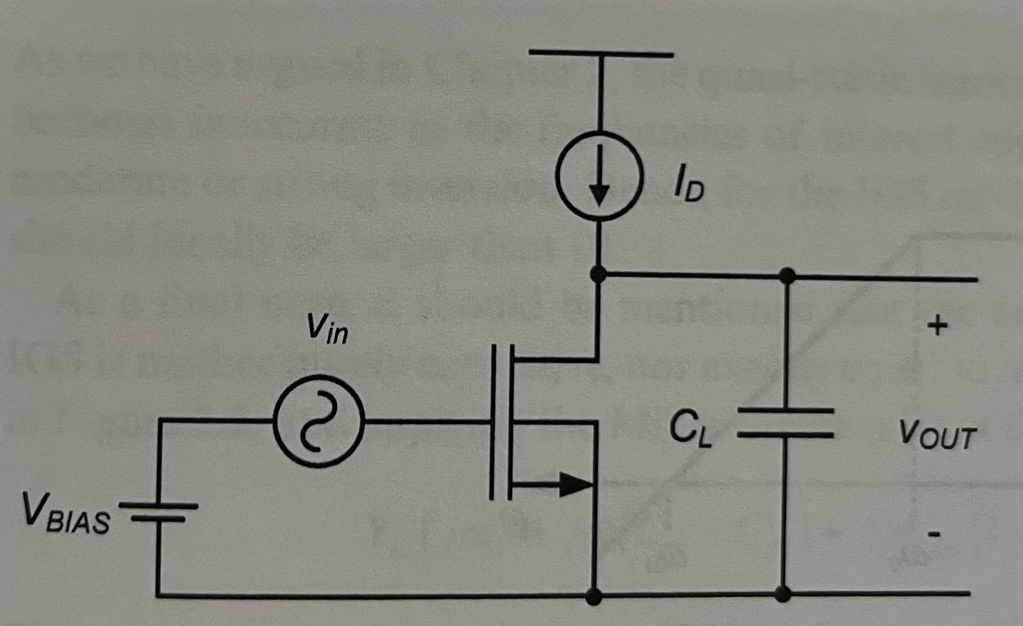
Circuit analysis#
If we insert the small signal model of the transitor into the above schematic, we get:
We’ll use some simplifiying assumptions:
\(C_{db} << C_L\)
\(C_{gd} << C_L\)
Junction capacitances can be ignored (for now)
Under those conditions, the frequency response can be approximated by:
Where:
and
Another thing to note is the unity gain frequency (\(\omega_u\)), given by:
It’s useful to measure the IGS’ fanout (FO), or the ratio of the capacitance it can drive to it’s input capacitance:
We could rewrite this as:
Because the quasi-static transistor model used above breaks down as frequency approaches about 1/10th of \(f_t\) in moderate or strong inversion, we want to keep FO > 10. (i.e., keep \(\omega_u\) under 1/10th of \(\omega_t\))
Sizing considerations#
So if we know the gain and frequency response, we want to do the following for some given combination of \(C_L\) and \(f_u\) target:
Find drain current
Find device length
Find device width
We can use this flow:
Determine \(g_m\) (from design specs)
Pick L:
Short channel: high speed, low area
Long channel: high intrinsic gain, improved matching
Pick \(g_m\over{I_d}\):
large \(g_m\over{I_d}\): low mpower, large signal swing (low \(V_{dsat}\))
small \(g_m\over{I_d}\): high speed, small area
Determine \(I_d\) (from \(g_m\) and \(g_m\over{I_d}\))
Determine W (from \(I_d\over{W}\))
If we are given a spec for \(\omega_u\), then \(g_m\) is fixed by \(\omega_u = \frac{g_m}{C_L}\).
But, we need more constraints to pick L and \(\frac{g_m}{I_d}\).
We could say that \(I_d = \frac{g_m}{g_m / I_d}\). Based on that, maybe we’d say we want to maximize \({g_m / I_d}\) to minimize drain current. But doing that requires a large device and a low \(f_t\), which may lead to violating the guideline that FO < 10.
This leads to the following: determining the right inversion level is complicated, and we need to take a lot of different factors into account. So we’re going to have to work out different constraints to help us pick a suitable inversion level.
For now, let’s talk about how to pick W given a L and \(g_m\over{I_d}\).
Sizing for given L and \(g_m\over{I_d}\)#
If we know those, finding W becomes:
We can call this flow “denormalization”, and it looks like this:
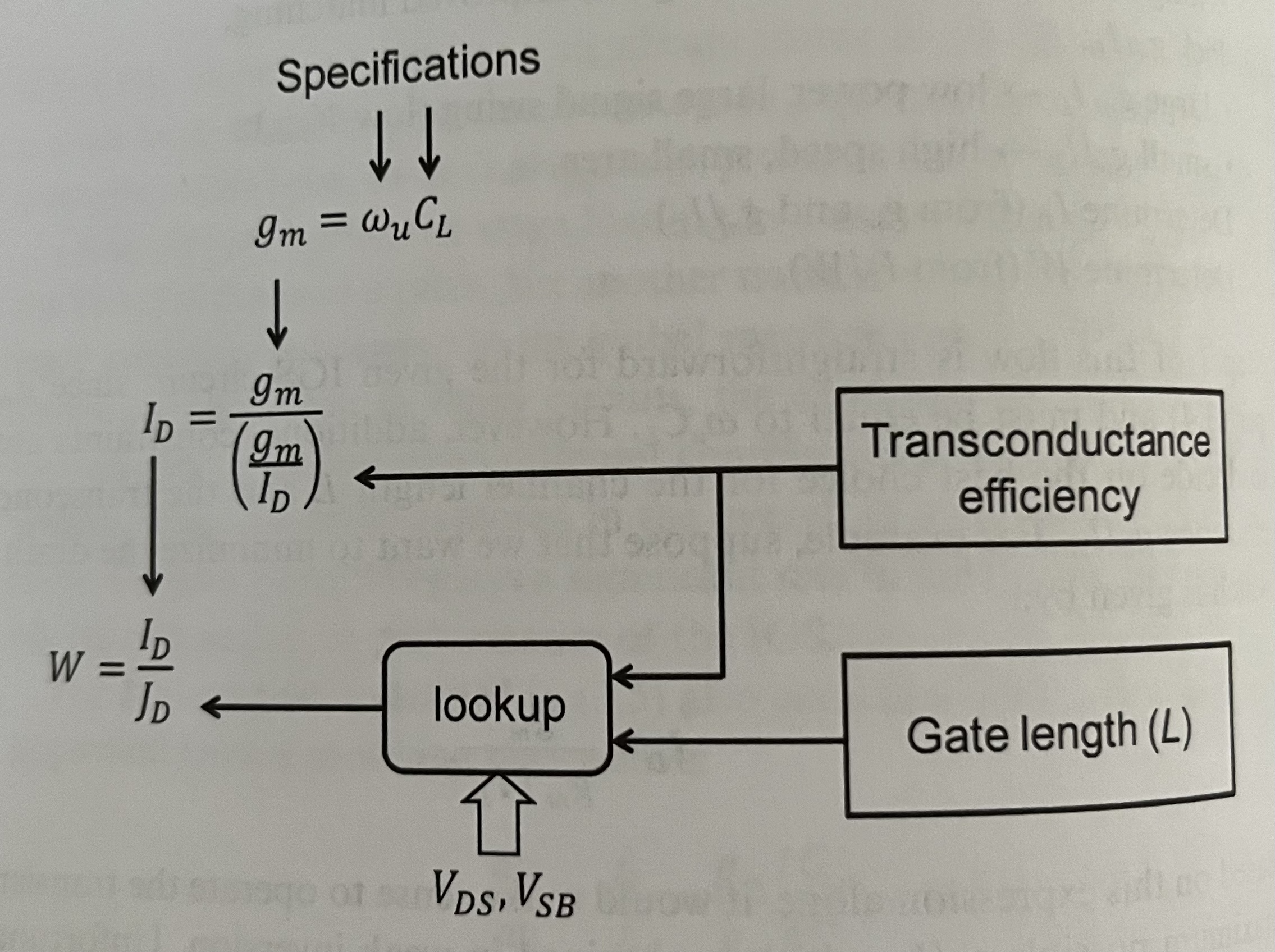
Once we know \(g_m / I_d\), L, \(V_{ds}\) and \(V_{sb}\), we can plug those into our lookup table and find the correpsonding \(J_d = I_d / W \). And when we know \(I_d\) from the required \(\omega_u\), \(C_L\) and \(g_m / I_d\), we can scale the W appropriately.
Note that we’re assuming that drain current scales linearly with width, which ignores narrow-width effects. If that doesn’t hold, we’d ideally have lookup tables with different widths and corresponding drain currents, or some non-linear scaling formula. This could be a good place to insert some ML; we could train a model to predict device performance based on physical parameters.
Let’s look at a concrete example…
Example: basic IGS sizing#
Suppose we want to design an IGS with:
\(f_u\) = 1 GHz
\(C_L\) = 1 pF
Assume:
L = 180nm
\(g_m / I_d\) = 15 S/A (moderate inversion)
\(V_{ds}\) = 0.6 V
\(V_{sb}\) = 0 V
Find the low frequency gain and the Early voltage of the transistor.
Solution:#
We’ll start by loading in our transitor data, supplied by Professor Murmann through his GitHub repo:
Show code cell source
# first, load up the nch dataset
nch_data_df = load_mat_data("../../Book-on-gm-ID-design-main/starter_kit/180nch.mat")
Loading data from ../../Book-on-gm-ID-design-main/starter_kit/180nch.mat
Found the following columns: ['ID', 'VT', 'GM', 'GMB', 'GDS', 'CGG', 'CGS', 'CGD', 'CGB', 'CDD', 'CSS', 'STH', 'SFL', 'INFO', 'CORNER', 'TEMP', 'VGS', 'VDS', 'VSB', 'L', 'W', 'NFING']
/Users/sean/.pyenv/versions/3.10.4/lib/python3.10/site-packages/pandas/core/internals/construction.py:576: VisibleDeprecationWarning: Creating an ndarray from ragged nested sequences (which is a list-or-tuple of lists-or-tuples-or ndarrays with different lengths or shapes) is deprecated. If you meant to do this, you must specify 'dtype=object' when creating the ndarray.
  values = np.array([convert(v) for v in values])
With that in place, we can look in our dataset to find transitors that match our givens, and interpolate for \(\frac{g_m}{I_d}\) = 15:
Show code cell source
# since we're given values for L, gm/Id, Vds and Vsb, I can lookup the associated Jd
# first, grab the subsection of data that matches the givens
biasing_mask = (
    (nch_data_df['VDS'] == 0.6) &
    (nch_data_df['VSB'] == 0.0) &
    (nch_data_df['L'] == 0.18)
    )

# now interpolate at gm/id = 15
lookup_df,interp_df = lookup(df=nch_data_df[biasing_mask], param='GM_ID', target=15)

cols = ['W', 'L', 'ID', 'GM', 'GM_ID', 'JD', 'VGS', 'VDS', 'VSB']
caption = "NMOS device data matching givens"

display(
    pretty_table(
        df=lookup_df,
        cols=cols,
        caption=caption
    )
    )
| W | L | ID | GM | GM_ID | JD | VGS | VDS | VSB |
|---|---|---|---|---|---|---|---|---|
| 5.000000 | 0.180 | 56.78u | 850.55u | 15 | 11.36u | 599.15m | 600.00m | 0.00m |
Since we know that \(f_u\) is 1 GHz and \(C_L\) is 1pF, we can derive the required \(g_m\):
Show code cell source
gm_spec = 2 * 3.14159 * 1e9 * 1e-12
print(f"The required gm is {gm_spec*1e3:.2f} mS")
The required gm is 6.28 mS
Given a \(g_m\over{I_d}\) of 15 and a \(g_m\) of 6.283e-3, our required drain current is:
Show code cell source
id_spec = gm_spec / lookup_df['GM_ID'].values[0]
print(f"The required drain current is {id_spec*1e6:.2f} uA")

scale_factor = id_spec / lookup_df['ID'].values[0]
print(f"This means we'll need to scale the device by {scale_factor:.2f}")
The required drain current is 418.88 uA
This means we'll need to scale the device by 7.38
Show code cell source
scaled_df = scale(
    df=lookup_df,
    scale_factor=scale_factor
)
cols=['W', 'L', 'ID', 'GM', 'GM_ID', 'JD', 'GDS',
      'CGG', 'CGS', 'CGD', 'VGS', 'VDS']
caption = "Scaled device dimensions and parameters"
display(pretty_table(
    df=scaled_df,
    cols=cols,
    caption=caption,
    transpose=True)
)
| W | 36.88 |
|---|---|
| L | 180.00m |
| ID | 418.88u |
| GM | 6.27m |
| GM_ID | 15.00 |
| JD | 11.36u |
| GDS | 170.57u |
| CGG | 74.44f |
| CGS | 52.80f |
| CGD | 17.84f |
| VGS | 599.15m |
| VDS | 600.00m |
Ok, now let’s calculate what the question actually asked for; intrinsic gain and early voltage:
Show code cell source
Av0 = -scaled_df['GM'].values[0] / scaled_df['GDS'].values[0]
print(f"The low frequency gain is {Av0:.2f}")

ft = scaled_df['GM'].values[0] / scaled_df['CGG'].values[0] / (2*3.14159)
print(f"The transit frequency is {ft/1e9:.2f} GHz")
The low frequency gain is -36.78
The transit frequency is 13.41 GHz
And remember that Early voltage is defined as:
Show code cell source
early_voltage = scaled_df['ID'].values[0] / scaled_df['GDS'].values[0]
print(f"The early voltage is {early_voltage:.2f}")
The early voltage is 2.46
Tradeoff exploration#
What happens if we don’t assume \(g_m\over{I_d}\) and L?
Let’s plot intrinsic gain and transit frequency vs. \(g_m\over{I_d}\) and L:
Show code cell source
TOOLTIPS = [
            ("x", "$x"),
            ("y", "$y")
        ]

# first, select the data that we want:
length_filter = [0.180, 0.240, 0.300, 0.360]
length_colors = {
    0.180: "blue",
    0.240: "green",
    0.300: "yellow",
    0.360: "red"
}
tradeoff_mask = ((nch_data_df['VDS'] == 0.6) &
                 (nch_data_df['VSB'] == 0) &
                 (nch_data_df['L'].isin(length_filter))
                 )
tradeoff_df = nch_data_df[tradeoff_mask]

# create a figure
tradeoff_plot = bh.create_bokeh_plot(
    title="Intrinsic gain and transit frequency vs. gm/Id and L",
    x_axis_label="gm / Id (S/A)",
    y_axis_label="ft (GHz)",
    tooltips=TOOLTIPS,
    width=800,
)

# create a secondary y-axis
tradeoff_plot.extra_y_ranges['gain'] = Range1d(0, 100)
ax2 = LinearAxis(y_range_name='gain', axis_label="Intrinsic Gain")
tradeoff_plot.add_layout(ax2, 'right')

# plot lines for each of the gate lengths we selected

for len, len_group in tradeoff_df.groupby('L'):
    data = ColumnDataSource(len_group)

    tradeoff_plot.line(x='GM_ID', y='GM_CGG', source=data,
                       legend_label=f"l={len}", line_color=length_colors[len])

    tradeoff_plot.line(x='GM_ID', y='GM_GDS', source=data,
                       y_range_name='gain', line_dash="dashed",
                       line_color=length_colors[len])

show(tradeoff_plot)
From the plot, we can see two things very clearly:
Transit frequency drops off with increasing \(\frac{g_m}{I_d}\)
Intrinsic gain trades off with transit frequency as we vary the device length
In general, we’ll have to manage these tradeoffs to meet design / system specs.
That’s where modeling comes in - we should explore how to budget the system through models and system-level simulations to help us hone in on how to balance [speed / gain / power / area / etc.]